Generative pixel images in Excel
This tutorial demonstrates how I
made generative art in Excel for a school project.
This is my second tutorial on the subject, in an attempt to improve the
readability based on feedback received.
I used Excel, but you should be able
to follow most of the steps in any other spreadsheet software.
I assume some basic knowledge of excel, such as how to resize cells, rename
sheets, entering formulas and conditional formatting.
The final export of images is made
automatic using VBA macros.
In this step, we set up an excel worksheet as the drawing area for our picture, by resizing the cells, adding a border around the drawing area and setting up conditional formatting rules.
First set up our drawing area
in excel, resize the rows and columns to be square in shape.
For BlockyBears, I set my cell size to 20 pixels x 20 pixels. Secondly, mark out a canvas for uour drawing.
Whether you have centralized parts to your drawing will affect whether you want
an odd number or event number of columns.

You can mark your border either with a single row of cells filled with a
colour, or using the cell outline tool.
For BlockyBears, I used a grid size of 63 rows x 63 columns.

Finally, select the entire drawing
area within the border created in step 2.
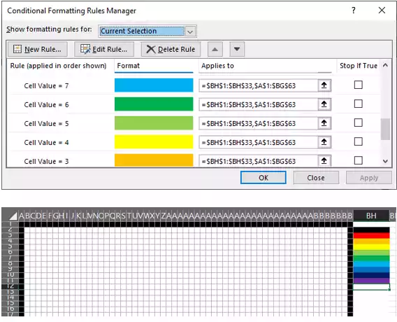
From the ribbon, select conditional formatting and new rule.
We will be formatting all cells
based on their value and assigning a colour to each value.
| Value | Colour |
|---|---|
| 0 | White |
| 1 | Black |
| 2 | Red |
| 3 | Orange |
| 4 | Yello |
| 5 | Light Green |
| 6 | Dark Green |
| 7 | Light Blue |
| ... | etc |
Within the conditional formatting
pop-up window
Set the rule type:
Format only cells that contain
Set the rule to be:
Cell value – Equal to – 0

Set both the cell fill colour and
fault colour to white.
Repeat this step for an assortment
of colours.
It is handy to also apply this
formatting to a selection of cells outside the drawing area so you can create a quick reference for yourself.
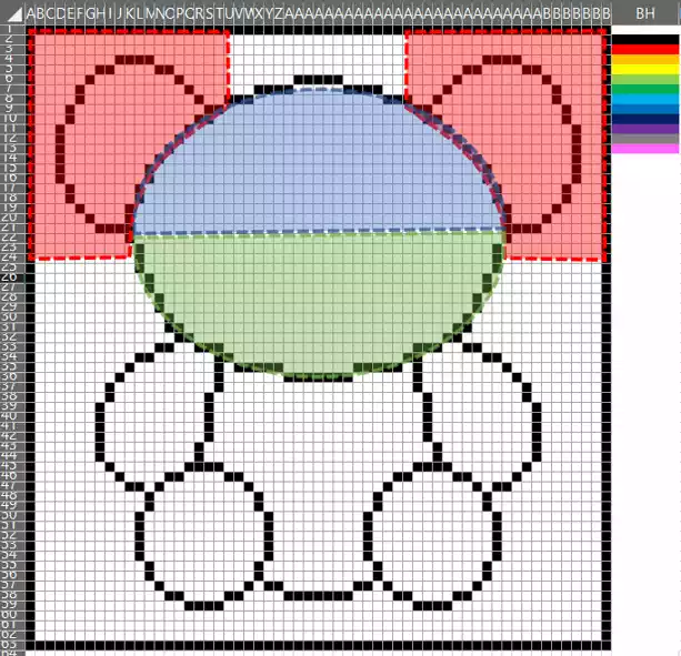
In this step, we draw the basic outline of our drawing from a sketch, without adding any additional features.
First either hand draw and scan, or
sketch using a drawing app the outline of your image.

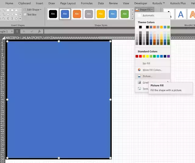
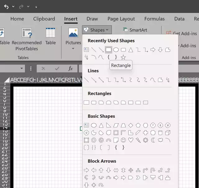
Using the excel drawing tools insert
a rectangle and resize this over your drawing area created in step 1.
Set the fill of this rectangle to be the picture file of your sketch and adjust
the transparency so you can see the cells beneath.
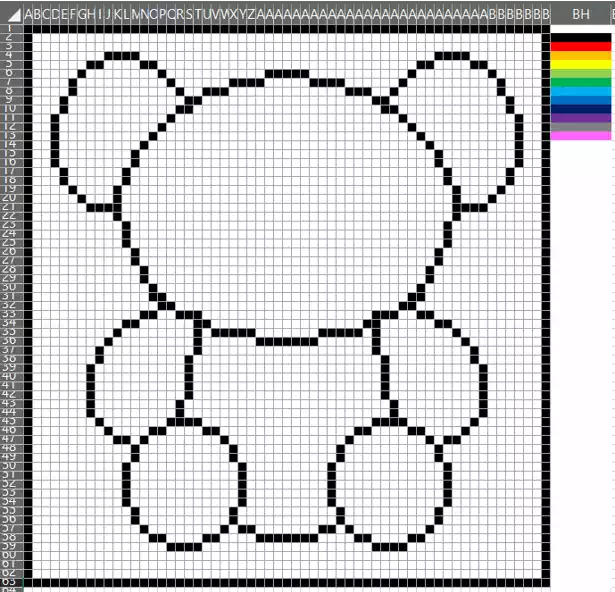
Follow the outline of the drawing,
typing "1" in each cell to set the cell to black using the
conditional formatting.

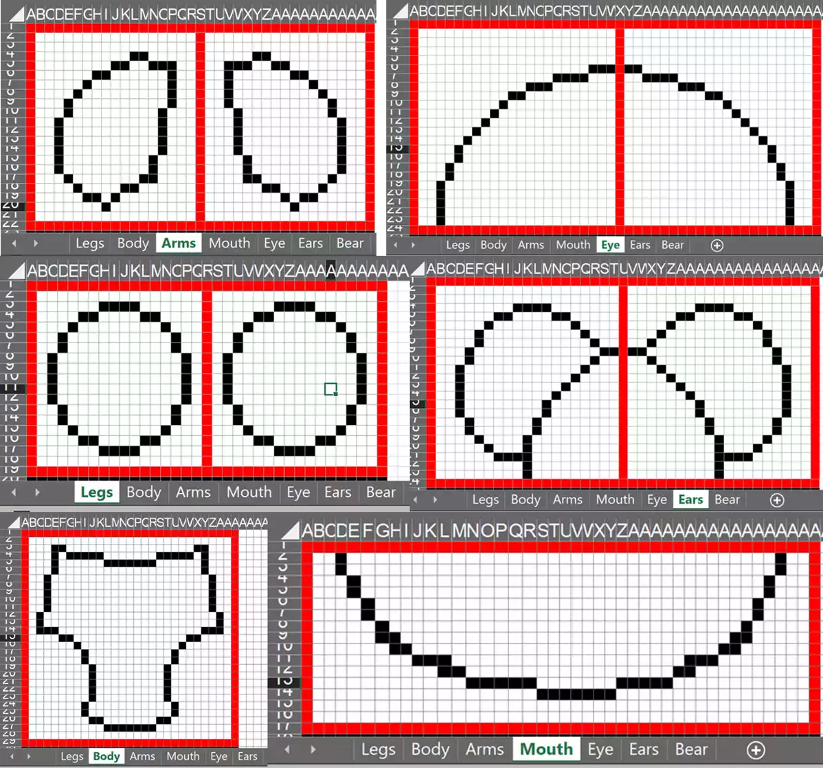
In this step, we break up the individual component features of our design that will be used to create the generated images.
Split
your drawing into the individual parts that you want to create individual
designs for.
BlockyBears is split into Ears, Eyes, Mouth, Body, Arms and Feet.
Create a new sheet in your workbook for each feature.
In each sheet, copy the features as
split up in step 3.
Make a mini-grid as per step 1 and set-up the conditional formatting.
Copy and paste the grid down the
sheet to make different versions.
Leave the first rows blank.
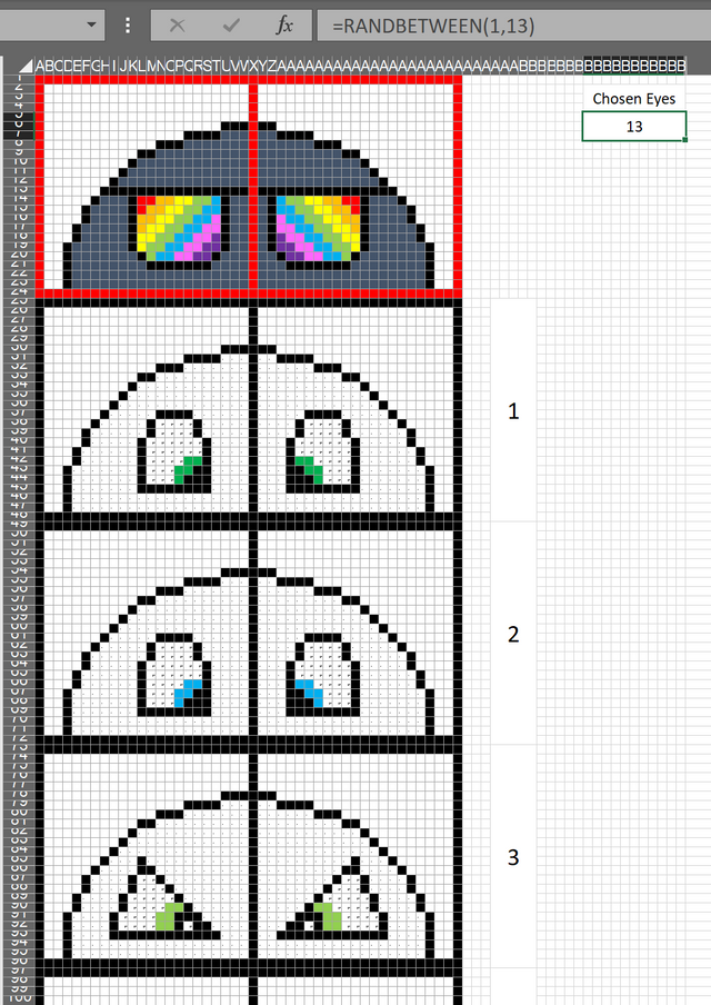
In this step, we design the individual features of our images.
Make your designs for each feature /
component of the image.
Use the units specified in the conditional formatting rules to make your designs
in each cell.
You can start with just 2 or 3 designs to skip to the next step, and go back to add more at a later date.

In this step, we lay down the ground rules for generating images. Initially this part is set up to require manual to show how everything works.
After designing all your features,
we need to be able to select each individual picture and change the image.
Add a box where you can type which legs to pick:
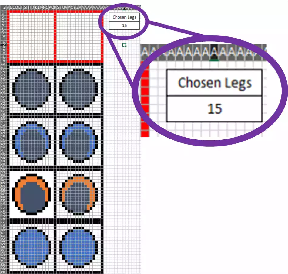
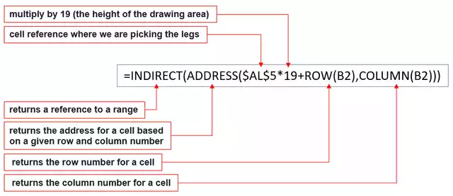
Inside the top cell (B2) of the drawing area add the following formula to copy the leg design selected:
=INDIRECT(ADDRESS($AL$5*19+ROW(B2),COLUMN(B2)))
Test that everything works by changing the value of the chosen feature (up to the maximum number of variations created)
Change the multiplication factor based on the number of rows in the drawing area. Copy the formula across to all other cells in the drawing area.
Repeat the process for all other
sections of your image on the other excel sheets creating each part of the
picture on its own sheet within the workbook.
Remember to modify the multiplication factor within the formula for different
sized features.
In this step, we lay modify our drawing canvas to bring in each the selected components from the individual feature sheets
After
finishing all the individual parts of your drawing, we need to put everything
back together in the main drawing.
Based on how the drawing was originally split into parts, link back each cell
to the cell on the corresponding feature sheet.
From the main drawing canvas, either
by typing “ = ” then clicking on the feature sheet and selecting the cell, or
by linking back to each sheet with the
formula:
=[SHEET_REFERENCE]!([CELL_REFERENCE])

In this step, we add the function to randomise our generated images
To randomize feature selection, go
back to the individual sheets where the chosen feature number is selected.
In the cell where you currently change the number add the formula:
=RANDBETWEEN(1,[MAX # OF FEATURES])
Substituting MAX # OF FEATURES for
the number of individual drawings created for that feature.
Each time Excel is refreshed, you
will be greeted by a new version of your drawing!
In this step, we output our images from excel. There are a few basic ways to do this for individual files.
The automated step is specifically for Excel 2019, though may work with earlier/later versions.
I explain the logic behind the export process, but you can skip straight to step 9 if you wish.
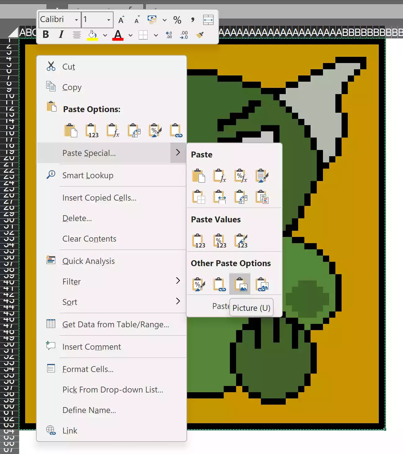
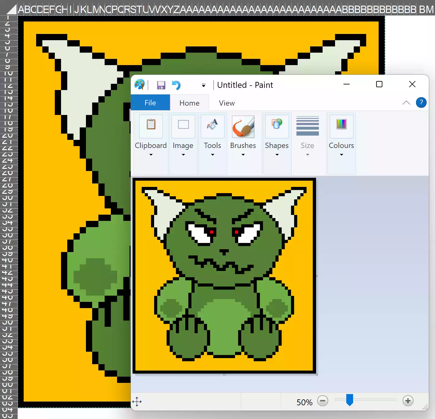
For the most basic way to ouput to an image file, select the drawing canvas, copy the area, then right click and "paste as picture".
You can also paste this selection directly into paint software such as MS Paint.
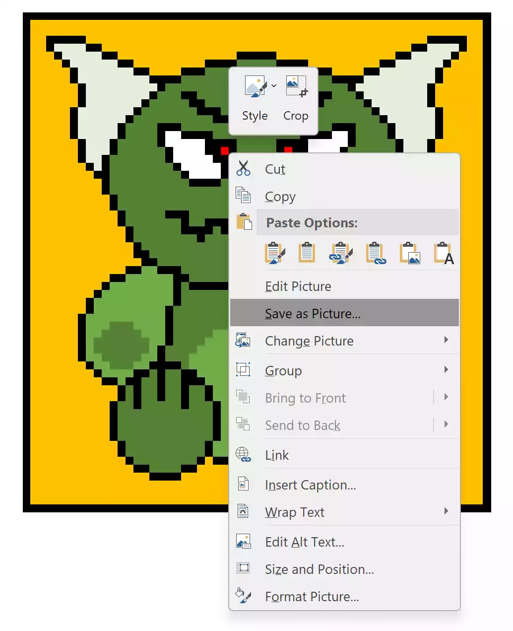
In some Microsoft office products, you can right click an image and "Save as Picture"
Unfortunately this is not a feature in Excel 2019, so I used a work-around.
Excel will allow a chart to be outputted to an image file with a macro.
Create a new sheet and insert a blank chart.
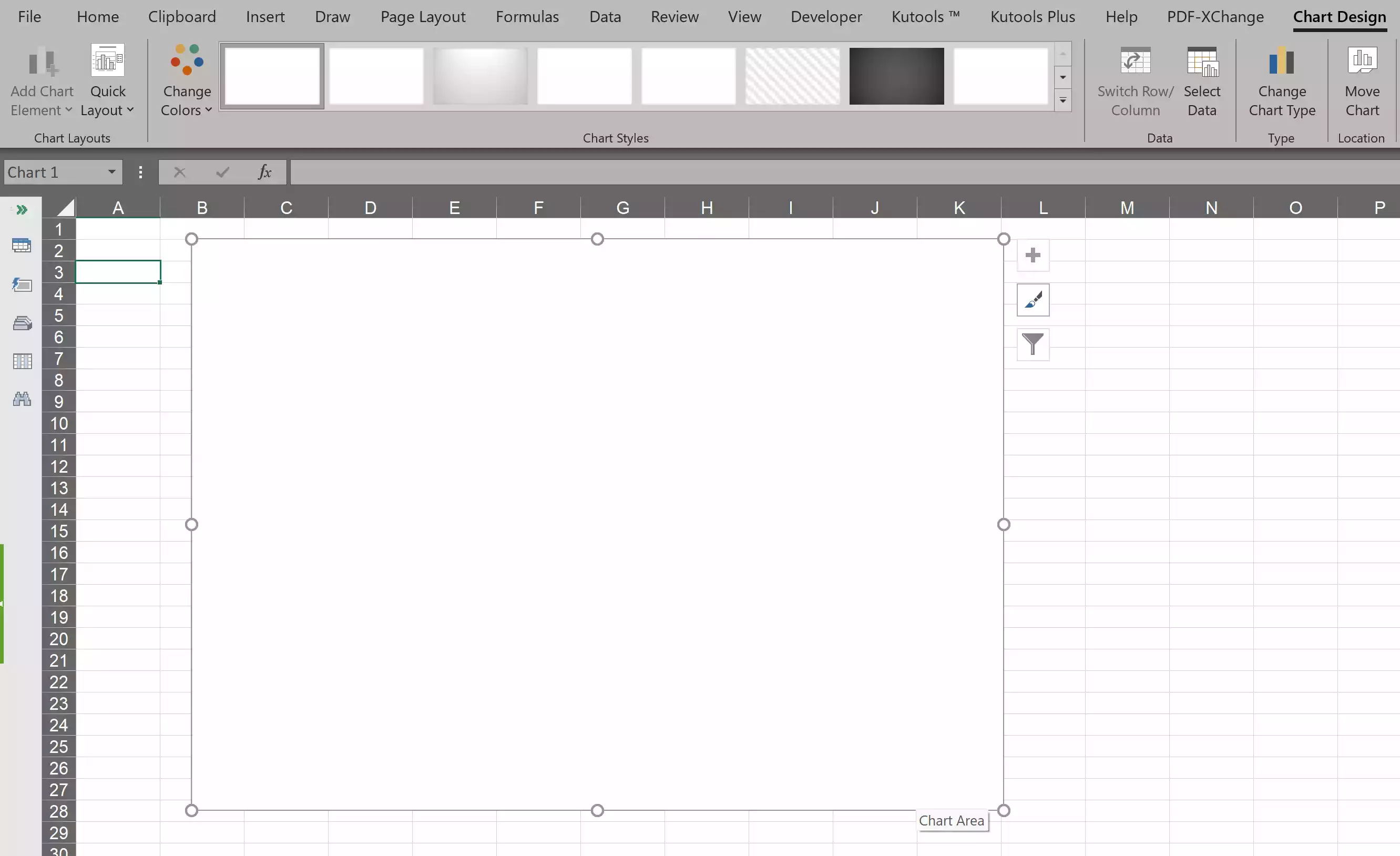

Within the chart area, paste in the picture (from the "paste as picture step")
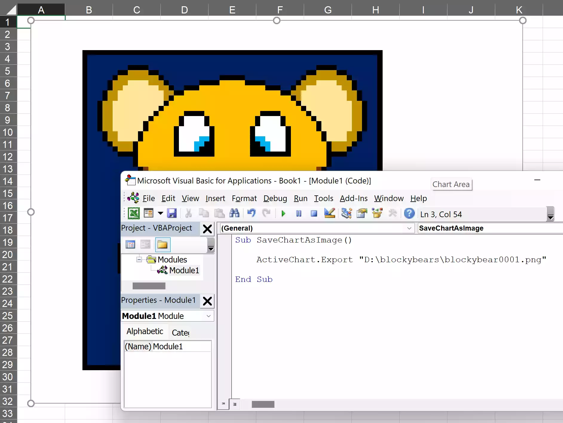
To export the chart area as an image, we need to create a VBA macro.
Switch to the developer tab and click on the Macros icon.
Give your macro a name, for example SaveChartAsImage the click create.
ActiveChart.Export "[Save Directory and Path]"
Set the outpath path and file name where you want to save your image.
You can output as an image type ie PNG, JPG, GIF.
After doing this, simply select the chart area and run the macro.
In this step, we automate output our images from excel. We jump straight into the process.
To generate a number of images, we can use a macro to automate the process of adding our image to a chart area and saving it to a folder.
Excel will automatically regenerate random numbers whilst the macro is running, which will create your new image.
The following macro will output 10 images, but will not prevent duplicate generations.
Check the inline comments to see what values need to be changed.
Sub exportimages()
''
'' Declare variables to use in the export process
''
Dim pic_rng As Range
Dim sh_temp As Worksheet
Dim ch_temp As Chart
Dim pic_temp As Picture
Dim pic_name As String
Dim save_directory As String
'' _________________________________________________________
''
'' Stop excel from updating the screen during the process to
'' save system memory resources
''
Application.ScreenUpdating = False
''
'' _________________________________________________________
''
'' Set folder where to save images
''
save_directory = "D:\blockybears\exports\" ' Change to your output folder
'' Set the cell range of the drawing area
''
Set pic_rng = Worksheets("Bear").Range("A1:BG63") ' Change to your drawing canvas area
'' Create a loop to generate as many images as you want
''
For i = 1 To 10 ' Change upper limit for more images
'' Set the picture name to the interation of the loop
''
pic_name = "image" & i & ".jpg"
'' Temporarily add a blank worksheet
''
Set sh_temp = Worksheets.Add
'' Add a blank chart to the new worksheet
''
Charts.Add
ActiveChart.Location where:=xlLocationAsObject, Name:=sh_temp.Name
'' Remove any formatting from the chart area
''
Set ch_temp = ActiveChart
ActiveSheet.Shapes(ActiveChart.Parent.Name).Line.Visible = msoFalse
'' Copy the drawing canvas as an image
''
pic_rng.CopyPicture appearance:=xlScreen, Format:=xlPicture
'' Paste the image into the blank chart
''
ch_temp.Paste
'' Resize the chart area to set the picture size
'' If your image is square set width and height the same
'' If you have made a rectangular shape canvas, adjust
'' Width and height to be a ration of one another
''
Set pic_temp = Selection
With ch_temp.Parent
.Width = 1024 ' Change for your preferred image size
.Height = 1024 ' Change for your preferred image size
End With
'' Export the image to the save directory
''
ch_temp.export Filename:=save_directory & pic_name
'' Disable excel prompts for deletion of the temp sheet
'' Delete the temp sheet
'' Re-enable excel prompts
''
Application.DisplayAlerts = False
sh_temp.Delete
Application.DisplayAlerts = True
Next i
'' Renable excel screen updates
''
Application.ScreenUpdating = True
End Sub